Silicon64
This example demonstrates a number of Qbox features in calculations of the electronic structure of a 64-atom bulk silicon sample.
The example includes:
Calculation of the ground state energy
Structure optimization
Molecular dynamics
Ground state energy calculation
Bulk silicon has a Face-Centered Cubic (FCC) unit cell containing two atoms. An 8-atom Simple-Cubic (SC) supercell can be formed by combining 4 replicas of the FCC primitive cell. The Si64 sample in turn consists of a 2x2x2 replication of the 8-atom SC cell.
Pseudopotential
The pseudopotential used for this example is defined in the file
Si_VBC_LDA-1.0.xml.
This file must be present in the current directory when running the first
electronic structure calculation of the Si64 sample.
Sample definition file
The sample is defined in the file
si64.i
where the unit cell is first defined using the set command and the
cell variable, the species ‘silicon’ is defined using the
species command, and
each atom is defined using the atom Qbox command.
set cell    20.52 0 0  0 20.52 0  0 0 20.52
species silicon Si_VBC_LDA-1.0.xml
atom Si01 silicon   -10.260000   -10.260000   -10.260000
atom Si02 silicon    -7.695000    -7.695000    -7.695000
atom Si03 silicon    -5.130000    -5.130000   -10.260000
atom Si04 silicon    -2.565000    -2.565000    -7.695000
atom Si05 silicon   -10.260000    -5.130000    -5.130000
atom Si06 silicon    -7.695000    -2.565000    -2.565000
atom Si07 silicon    -5.130000   -10.260000    -5.130000
atom Si08 silicon    -2.565000    -7.695000    -2.565000
atom Si09 silicon   -10.260000   -10.260000     0.000000
atom Si10 silicon    -7.695000    -7.695000     2.565000
atom Si11 silicon    -5.130000    -5.130000     0.000000
atom Si12 silicon    -2.565000    -2.565000     2.565000
atom Si13 silicon   -10.260000    -5.130000     5.130000
atom Si14 silicon    -7.695000    -2.565000     7.695000
atom Si15 silicon    -5.130000   -10.260000     5.130000
atom Si16 silicon    -2.565000    -7.695000     7.695000
atom Si17 silicon   -10.260000     0.000000   -10.260000
atom Si18 silicon    -7.695000     2.565000    -7.695000
atom Si19 silicon    -5.130000     5.130000   -10.260000
atom Si20 silicon    -2.565000     7.695000    -7.695000
atom Si21 silicon   -10.260000     5.130000    -5.130000
atom Si22 silicon    -7.695000     7.695000    -2.565000
atom Si23 silicon    -5.130000     0.000000    -5.130000
atom Si24 silicon    -2.565000     2.565000    -2.565000
atom Si25 silicon   -10.260000     0.000000     0.000000
atom Si26 silicon    -7.695000     2.565000     2.565000
atom Si27 silicon    -5.130000     5.130000     0.000000
atom Si28 silicon    -2.565000     7.695000     2.565000
atom Si29 silicon   -10.260000     5.130000     5.130000
atom Si30 silicon    -7.695000     7.695000     7.695000
atom Si31 silicon    -5.130000     0.000000     5.130000
atom Si32 silicon    -2.565000     2.565000     7.695000
atom Si33 silicon     0.000000   -10.260000   -10.260000
atom Si34 silicon     2.565000    -7.695000    -7.695000
atom Si35 silicon     5.130000    -5.130000   -10.260000
atom Si36 silicon     7.695000    -2.565000    -7.695000
atom Si37 silicon     0.000000    -5.130000    -5.130000
atom Si38 silicon     2.565000    -2.565000    -2.565000
atom Si39 silicon     5.130000   -10.260000    -5.130000
atom Si40 silicon     7.695000    -7.695000    -2.565000
atom Si41 silicon     0.000000   -10.260000     0.000000
atom Si42 silicon     2.565000    -7.695000     2.565000
atom Si43 silicon     5.130000    -5.130000     0.000000
atom Si44 silicon     7.695000    -2.565000     2.565000
atom Si45 silicon     0.000000    -5.130000     5.130000
atom Si46 silicon     2.565000    -2.565000     7.695000
atom Si47 silicon     5.130000   -10.260000     5.130000
atom Si48 silicon     7.695000    -7.695000     7.695000
atom Si49 silicon     0.000000     0.000000   -10.260000
atom Si50 silicon     2.565000     2.565000    -7.695000
atom Si51 silicon     5.130000     5.130000   -10.260000
atom Si52 silicon     7.695000     7.695000    -7.695000
atom Si53 silicon     0.000000     5.130000    -5.130000
atom Si54 silicon     2.565000     7.695000    -2.565000
atom Si55 silicon     5.130000     0.000000    -5.130000
atom Si56 silicon     7.695000     2.565000    -2.565000
atom Si57 silicon     0.000000     0.000000     0.000000
atom Si58 silicon     2.565000     2.565000     2.565000
atom Si59 silicon     5.130000     5.130000     0.000000
atom Si60 silicon     7.695000     7.695000     2.565000
atom Si61 silicon     0.000000     5.130000     5.130000
atom Si62 silicon     2.565000     7.695000     7.695000
atom Si63 silicon     5.130000     0.000000     5.130000
atom Si64 silicon     7.695000     2.565000     7.695000
Note
The size of the unit cell and the position of the atoms must be specified in atomic units (bohr).
The calculation of the electronic ground state is done using the
Qbox script si64gs.i
1si64.i
2set ecut 12
3set wf_dyn PSDA
4set scf_tol 1.e-6
5randomize_wf
6run 0 30 10
7save si64gs.xml
In line 1, the script
si64.iis invoked and the contents of the script are executed, defining the unit cell, the speciessiliconand the position of all atoms.Line 2 defines the plane wave energy cutoff ecut to be 12 Ry. This resizes the plane wave basis set accordingly. Note that the unit used for the plane wave energy cutoff (Rydberg) is an exception to the convention used otherwise in Qbox to use atomic units (Hartree and bohr).
Line 3 defines the algorithm used to update wave functions by setting the variable wf_dyn to
PSDA(Preconditioned Steepest Descent with Anderson acceleration).Line 4 defines the tolerance used to determine convergence in self-consistent iterations (variable scf_tol). Iterations are considered converged when the energy changes by less than 10-6 (hartree).
Line 5 uses the randomize_wf command to add random numbers to the electronic wave function coefficients before starting the calculation. This is necessary to avoid spurious stationary points in the optimization for systems of high symmetry (such as bulk silicon).
Line 6 invokes the run command to perform the calculation. The first argument (0) refers to the number of ionic steps (during which the atoms are moved). This is zero for the present calculation since we are only optimizing the electronic wave functions with fixed atoms. The second argument (30) is the maximum number of self-consistent iterations performed. The actual number of iterations may be smaller if the convergence criterion scf_tol is reached before 30 iterations. The third argument (5) is the number of iterations used to update wave functions between updates of the charge density.
Line 7 uses the save command to save the description of the current system (atomic species, atomic positions and wave functions) on file
si64gs.xmlfor later use in other calculations.
The calculation can be run by invoking Qbox as:
$ mpirun -np 2 qb si64gs.i > si64gs.r
Structure optimization
This section describes an example of structure optimization.
The calculation starts from the previously saved file si64gs.xml
that contains the results from the above
electronic ground state calculation.
The atomic positions defined in the file si64.i correspond to the
equilibrium positions in the crystal. Running a structure optimization
in that structure would not show any change in the atomic positions since
the system is already in an energy minimum. For this reason, we first
impose an arbitrary displacement to two atoms. We then recompute the
electronic ground state in the displaced configuration. Finally we run
the structure optmization. We choose to displace the atom Si57
(originally located at (0,0,0)) in the (1,1,1) direction. Furthermore, we
displace the atom Si58 (initially located at (2.56,2.56,2.56)) in the
opposite direction. This displacement amounts to compressing the
covalent bond between Si57 and Si58. We also print the
distance between Si57 and Si58 before and after the displacement.
The complete procedure is included in the
Qbox script si64cg.i
 1load si64gs.xml
 2# print Si57-Si58 distance
 3distance Si57 Si58
 4# displace atoms
 5move Si57 by  0.1  0.1  0.1
 6move Si58 by -0.1 -0.1 -0.1
 7distance Si57 Si58
 8# recompute the ground state
 9set wf_dyn PSDA
10set scf_tol 1.e-6
11run 0 20
12# optimize the geometry again
13set atoms_dyn CG
14run 20 20
In line 1, the sample restart file saved in the previous ground state calculation is loaded using the load command. Note that it is not necessary to perform the ground state calculation as a separate run. The contents of the file
si64gs.icould be included to replace line 1 if a single run is desired.Line 3 computes and prints the distance between atoms
Si57andSi58in their original equilibrium positions.Lines 5 and 6 use the move command to displace the atoms
Si57andSi58using relative displacements.Line 7: The distance is printed again after the displacement.
Lines 9-11: The electronic ground state is recomputed in the displaced configuration.
Line 13: The Conjugate Gradient (CG) algorithm is chosen for the atomic motions during the structure optimization (variable atoms_dyn).
Line 14: Run 20 steps of CG optimization with up to 20 self-consistent iterations after each CG step.
The structure optimization can be run using e.g. the command:
$ mpirun -np 2 qb si64cg.i > si64cg.r
This calculation results in the structure relaxing back to its original
geometry. The position of the Si57 atom can be monitored using the
following xml_grep command:
$ xml_grep 'atom[@name="Si57"]' sicg64.r
Note the use of XPath syntax for the selection of the contents. If we only
want to extract the <position> element of this atom, we can use:
$ xml_grep 'atom[@name="Si57"]/position' sicg64.r
which results in the output
<?xml version="1.0" ?>
<xml_grep version="0.9" date="Wed Sep 19 10:56:30 2018">
<file filename="si64cg.r">
<position> 0.10000000 0.10000000 0.10000000 </position>
<position> 0.10000000 0.10000000 0.10000000 </position>
<position> 0.07091875 0.07091496 0.07091517 </position>
<position> 0.03892938 0.03892141 0.03892186 </position>
<position> 0.03272656 0.03272011 0.03272313 </position>
<position> 0.02590347 0.02589868 0.02590453 </position>
<position> 0.01315803 0.01315262 0.01315769 </position>
<position> 0.00971123 0.00970692 0.00971360 </position>
<position> 0.00591369 0.00590986 0.00591650 </position>
<position> 0.00437996 0.00437665 0.00438359 </position>
<position> 0.00304774 0.00304471 0.00305234 </position>
<position> 0.00230019 0.00229737 0.00230545 </position>
<position> 0.00175876 0.00175604 0.00176424 </position>
<position> 0.00148228 0.00147959 0.00148851 </position>
<position> 0.00115785 0.00115514 0.00116439 </position>
<position> 0.00099169 0.00098897 0.00099865 </position>
<position> 0.00090564 0.00090294 0.00091274 </position>
<position> 0.00077748 0.00077469 0.00078462 </position>
<position> 0.00072244 0.00071967 0.00072987 </position>
<position> 0.00061519 0.00061231 0.00062260 </position>
<position> 0.00058607 0.00058320 0.00059378 </position>
</file>
</xml_grep>
Similarly, the evolution of the force on atom Si57 can be extracted
using:
$ xml_grep 'atom[@name="Si57"]/force' si64cg.r
The distance between Si57 and Si58 can be extracted using one of
the Qbox utility scripts (in the util directory):
$ qbox_distance.py Si57 Si58 si64cg.r
This shows that the distance has relaxed to the value 4.441 (bohr), close to the original equilibrium distance of 4.443 (bohr).
Molecular dynamics
In this example, we demonstrate a molecular dynamics simulation. We start
from the previously computed electronic ground state saved in the
restart file si64gs.xml. Rather than imposing arbitrary displacement
on atoms, we set the initial atomic velocities to be randomly sampled
from a Maxwell-Boltzmann distribution at a temperature of 300 K.
We then choose Molecular Dynamics (MD) as the
algorithm for atomic motions. A time step must also be chosen for the
numerical integration of the Newton equations of motion.
The complete MD simulation is included in the
Qbox script si64md.i
1load si64gs.xml
2# randomize velocities
3randomize_v 300
4set scf_tol 1.e-6
5# run 100 MD steps
6set dt 40
7set atoms_dyn MD
8run 100 20
In line 1, the sample restart file saved in the previous ground state calculation is loaded using the load command.
In line 3, the atomic velocities are randomized using the randomize_v command. The argument (300) is the temperature of the Maxwell-Boltzmann distribution from which velocities are drawn.
Line 4 defines the tolerance used for the convergence of the self-consistent iterations.
Line 5: A time step of 40 (a.u.) (approximately 0.968 fs) is chosen for the integration of the atomic equations of motion.
Line 6: The Molecular Dynamics (MD) algorithm is chosen for the atomic motions during the simulation. This uses the Verlet algorithm to update atomic positions at each time step.
Line 7: Run 100 MD steps, with up to 20 self-consistent iterations after after each step.
The MD simulation can be run using e.g. the command:
$ mpirun -np 2 qb si64md.i > si64md.r
Once the simulation is completed, the evolution of the Kohn-Sham energy and the quality of energy conservation can be visualized using:
$ econste.plt si64md.r
resulting in the following image
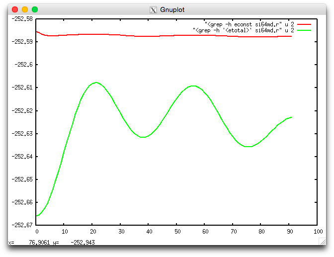
Fig. 6 Kohn-Sham energy <etotal> (green) and constant of the motion <econst> (red) during the molecular dynamics simulation.
This shows that the constant of the motion <econst> is reasonably constant on the scale of the fluctuations of <etotal>.